NX 5 Response Analysis Random Response

本文摘要（由AI生成）：

本文介绍了如何通过一系列步骤进行信号处理和分析。首先，在XY绘图编辑模式下，编辑X轴范围并设置频率限制。接着，比较原始PSD响应和由瞬态响应计算得到的PSD响应的RMS值。文中还提到了使用函数数学运算进行PSD的“清理”，生成移动平均值。最后，绘制原始PSD响应和移动平均操作生成的函数，并总结了整个工作流程。

This workshop demonstrates NX 5 Response Analysis capability for analyzing the dynamic response of a motorcycle fender. A Power Spectral Density (PSD) random excitation will be defined in the Function Toolkit.

This PSD acceleration function will be applied in the workshop as enforced motion loading on the fender at the connection to the fork. We want to evaluate the dynamic displacements and stresses in the fender.

The PSD excitation will also be converted to a transient excitation and the solution re-solved in the time domain. Conversion to time domain is useful if one wants to perform a fatigue analysis of what is an inherently random loading since most fatigue software operates on time domain data. Also if frequency loads (such as from an engine), and random loads (such as from road input), occur at the same time, it is not possible to combine them in the frequency domain, but you can in the time domain. 

Steps of Workshop:

·        Set Role

·        Open .prt file

·        Create a fem

·        Generate a Mesh

·        Create a simulation

·        Define boundary conditions

·        Define solver parameters

·        Solve for Modes UsingNX NastranSolver

·        Post Process the Results to View the Mode Shapes

·        Create Response Simulation

·        Define Random Excitation Function

·        Create Response Simulation Event for a Random Excitation

·        Compute Response Functions for the Random Event

·        Compute Full Field Response for the Random Event

·        Convert PSD excitation to Transient

·        Create Response Simulation Event for Transient Excitation

·        Compute Response Functions for the Transient Event

·        Convert Transient Results to PSD

·        Compare PSD event Results to Transient Results

Set Role

Start NX 5. Select the ‘Roles’ tab on the resource bar ()

· Set the role to ‘Advanced with full menus’

Open the .prt File

Select “File, open” to open “fender.prt”.

·        Set ‘Files of type’ to “Part Files (*.prt)”

·        Navigate to the appropriate folder and select ‘fender.prt’

·        Select ‘OK’

The part file contains a sheet body of the fender and a point located at the center of the four mounting holes.

Create a new FEM model

Start Advanced Simulation

Open the Simulation Navigator

Right click on fender.prt and select ‘New FEM…’. Name the new  fem fender_fem’

On the New FEM form:

• Toggle on ‘Associate to part’ and ‘Create Idealized Part’

• Select ‘Use all bodies’

• Open ‘Geometry Options…’ and select ‘All On’. Click ‘OK’

• This will include the point in the Idealized part and the FEM

• Click ‘OK’ to create the FEM

Generate Mesh

Generate a 2D Mesh on all of the surfaces in the polygon body

• Set an overall element size of 8.0 mm

This will create a 2D collector container and a thin shell collector (ThinShell(1)) for the mesh.

Right click on the ThinShell(1) collector and pick ‘Edit…’

• Note that a physical property table named ‘PSHELL1’ was created     and assigned.

Select the Modify button to modify this table

• Note that the PSHELL1 table has material set to ‘Inherited’ and     not thickness defined.

• There is no material associated to the part, so there is no material     to inherit

• Select choose material

• Retrieve material 13 (STEEL) from the Library

• Return to the PSHELL form and verify that Material 1 is set to     STEEL

• Set the Default Thickness to 1.0 mm 

• Click ‘OK’ on the PSHELL form and the Mesh Collector form to     complete the assignment of material and physical properties to the shell     mesh.

Create a 1D mesh of RBE2 elements between the point and the 4 circular edges of the mounting holes

• Select the point in Group 1

• Select the 4 circular edges in Group 2

There are no properties to define for rigid elements. This completes the mesh for the fender

 Create a Simulation

Right click on the fender_fem in the Simulation Navigator and select “New Simulation”.

·        Enter a new filename of ‘fender_sim.sim’

·        Select ‘OK’

·        Hit ‘OK’ on the New Simulation form:

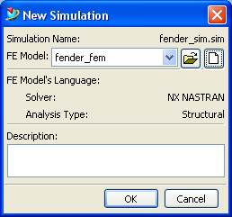
·        Change the Solution Type to ‘SEMODES 103 – Response Simulation’ on the Create Solution form.

·        Modify the name of the solution if you wish

·        Select ‘OK’

·        The result is a new simulation that contains an empty Response Simulation solution

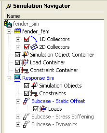
Define Boundary Conditions

The input for this analysis is a displacement time history measured during a rough road test. The nodes at the input location must be marked as enforced motion locations so that theNX Nastransolution output includes the necessary constraint modes.

·        Node display may be off by default in the new sim file. In order to define boundary conditions on nodes, they must be visible.

o   Select ‘Preferences, Node and Element Display…’ on the menu bar.

o   Set the Node Marker to ‘Dot’ (or asterisk if you prefer)

o   Select ‘OK’

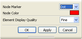
·        Right click on ‘Constraints’ under the Response Simulation solution

·        Select ‘New Constraint’, ‘Enforced Motion Location’

·        Select the node at the center of the rigid elements

·        Set all 6 DOF to ‘Enforced;

·        Change the default name if you wish

·        Select ‘OK’

·        This will fix the grid in all 6 degrees of freedom for the modal analysis via an SPC. It will also place the 6 degrees of freedom in the U2 USET, which will tell the solver to generate a constraint mode for each of the dof.

Define Solver Parameters

Prior to solving, the solution parameters need to be defined to tell the solver how many modes and/or what frequency range to solve for, as well as what output to recover.

When the Response Simulation solution was created, three subcases were automatically defined: one for Static Offset; a second for Stress Stiffening and a third for Dynamics. This analysis does not contain a Static offset or Stress Stiffening, so only the attributes for the Dynamics subcase need to be defined.

·        Right click on ‘Subcase – Dynamics’ in the Simulation Navigator and select ‘Edit Attributes…’ to bring up the Edit Solution Step form

·        Select the Open Manager button next to Output Requests (boxed in red above) to open the Modeling Objects Manager

·        Select Create

·        On the Stress tab, change the location from ‘CENTER’ to ‘CORNER’

·        Cycle through all of the remaining tabs except for Displacement and SPC Forces and toggle off the ‘Enable XXXXX Request’ checkbox on each tab.

·        Select ‘Preview’ and verify that the output requests match the following:

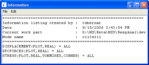
·        Close the Preview window and select OK on the Structural Output Request form and Close on the Modeling Objects Manager form

·        Select the Open Manager button next to Lanczos Method (boxed in magenta in the Edit Solution Step image above) to open the Modeling Objects Manager

·        Select Create

·        Define a frequency range of 0 to 1024 Hz

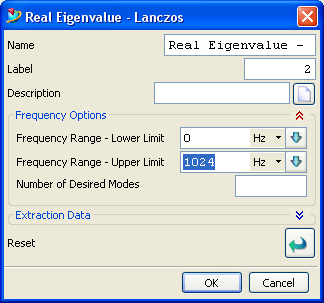
·        Select OK on the Real Eigenvalues form and Close on the Modeling Objects Manager Form

·        The objects just created should be selected in the drop down menus on the Edit Solution Step form:

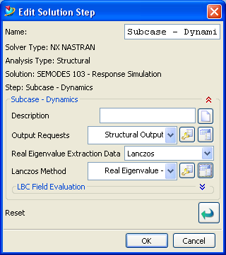
·        Hit OK

Solve for Modes UsingNX NastranSolver

Right click on the Response Simulation solution in the Simulation Navigator and select ‘Solve…’

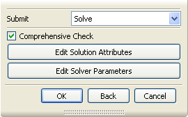
·        Hit OK

Post Process the Results to View the Mode Shapes

·        When the solution is completed, a Results item will appear in the Simulation Navigator under the Response Simulation Solution. Double click on Results to switch to the Post Processing Navigator and load the results.

OR…

·        Select the Post Processing Navigator tab () on the Resource Bar. Double click on the Response Simulation solution (or right click and select ‘Load’) to load the results. Once they are loaded, expand the list to see all the modes:

·        You should see that there are 18 mode shapes from 20.25 Hz to 972.1 Hz.

·        There are also 6 constraint modes, one for each enforced motion degree of freedom

·        Expand the results list for Mode 1 by clicking the ‘plus’ () to the left.

·        Double click on the ‘Displacement – Nodal’ item (or right click and select PLOT) to plot the mode shape.

·        Toggle on the Post-Processing toolbar (if it isn’t already on):

·        Use the red arrow to animate the mode shape. Use the green arrows to activate different modes. Look at several modes to see if they look reasonable.

·        Select ‘Return to Model’ () on the layout toolbar when finished viewing the mode shapes to close post processing.

Create Response Simulation

·        Return to the Simulation Navigator tab on the Resource Bar

·        Toggle on the Response Simulation toolbar (if it isn’t already on):

·        Select the ‘Create Response Simulation’ icon

·        On the Create Response Simulation form, enter a name if you wish and select the ‘Response Sim’ Response dynamic solution.

·        Select OK

This will create a Response Simulation item in the Simulation Navigator:

Notice that the modal representation for this analysis consists of the 18 normal modes plus an additional 6 constraint modes (one constraint mode shape is stored for each enforced motion location that was defined in the Response Simulation solution).

·        Mode shapes may also be plotted by right clicking on the Normal Modes or Constraint Modes items and selecting ‘Quick View’.

·        For a summary of the Normal Modes, click on the ‘Response Simulation Details View’ tab at the bottom of the Simulation Navigator

o   This summary includes modal mass, stiffness and damping for each mode

Define Random Excitation Function

Open the Function Manager ()

This function will be created as a table in an .afu file

• Set Purpose to ‘Response Simulation’

• Set Function Type to ‘Power Spectral Density (PSD)’

• Select New ()

On the ID page of the XY Function Editor:

• Enter a new AFU File name (i.e. fender_PSD.afu)

• Enter a name of ‘RoadVibrationY’ for the record name

On the XY Axis Definition page:

• Set Abscissa Spacing to ‘Uneven’

• Abscissa Data Type and Unit should be already be set to      Frequency and Hz

• Set Ordinate Data Type to ‘Acceleration’

• Set Ordinate unit to ‘g’

On the XY Data page, select to key in data from the list window

Enter the following data points:

Click ‘OK’ to create the function

Click ‘OK’ to close the XY Function Manager form

Plot the PSD excitation function

• Open the XY Function Navigator

• Expand the Associated AFU item

• The fender_PSD afu we created is associated to the current      simulation

• Expand the fender_PSD item

• The RoadVibrationY function just entered is located here

• Right click on RoadVibrationY and select ‘Plot’(XY)

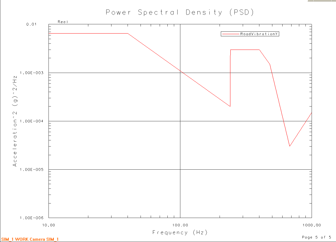
You can use the XY Graph toolbar () to toggle on edit mode to modify curve style, labels (text & fonts), X and or Y axis zoom, etc.

Create Response Analysis Event for a Random Excitation

·        Right click on the Response Simulation item in the Simulation Navigator and select ‘Create Event’ or use the Create Event icon ()on the Response Analysis toolbar.

·        Set event type to ‘Random’

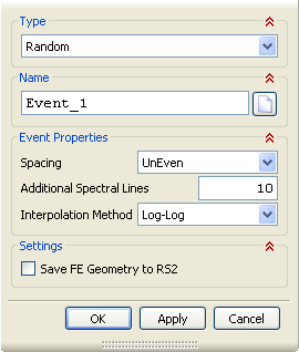
·        Select OK

·        This will create an event item in the Simulation Navigator

·        Right click on the Excitations item and select ‘Create Translational Nodal Excitation’ or use the () icon on the Response Analysis toolbar

·        Set the type to Enforced Motion

·        Using the List Selection or Graphic Selection method, select the independent grid of the RBE2 element

o   This is the only node that had an enforced motion location defines in the Response Analysis solution. It is the only item in the selection list and the only node that is selectable in the graphic display.

·        Toggle off the checkbox for the X and Z excitation functions. Using the button, open the function manager to select the RoadVibrationY function for the Y excitation.

·        Select OK

Next, apply damping to the modes of the event.

·        Right click on the Normal Modes item and select ‘Edit Damping Factor’

 ·        Specify 3% viscous damping on all modes

·        Select OK

·        Note: For more detailed control (activate/deactivate individual modes, specify different damping values for different modes, etc.) use the ‘Response Simulation Details View’. One or more modes can be selected using standard <Ctrl>/<Shift> list selection. Right click to modify.

Compute Response Functions for the Random Solution

·        In the Simulation Navigator, right click on the event and select ‘Solve for Modal Response’.

o   This will generate an event evaluation file (.eef) containing the modal response of the model to the defined input.

o   Note that this step is “optional”. The Modal Response will be solved for automatically the first time you evaluate a response if this step is skipped.

·        Right click on the event, then on Evaluate Function Response and pick ‘Nodal Function’.

·        Set the Result Type to ‘Acceleration’

·        Select the grid on the –X end of the fender at the vertex shared by 3 edges as shown below

·        Set the Data Component to Y

·        Toggle on Store to AFU to permanently store the response function in an external AFU file.

·        Select OK

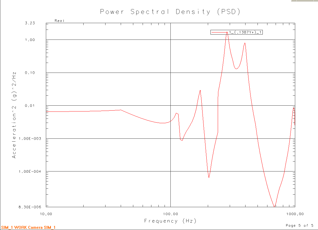
·        Plot the generated response function together with the input function

·        The result should look like:

Now, generate functions for elemental results such as stress.

·        Right click on the event, then on Evaluate Function Response and pick ‘Elemental Function’.

·        Set the Result Type to Stress

·        Select an element near the center of the strut as shown below

·        Set the Data Component to Von Mises

·        Toggle on Store to AFU to permanently store the response function in an external AFU file.

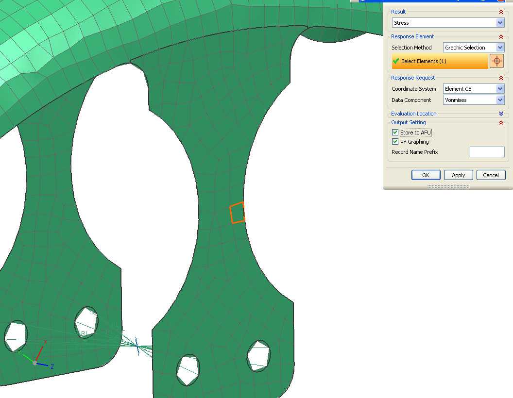
·        Select OK

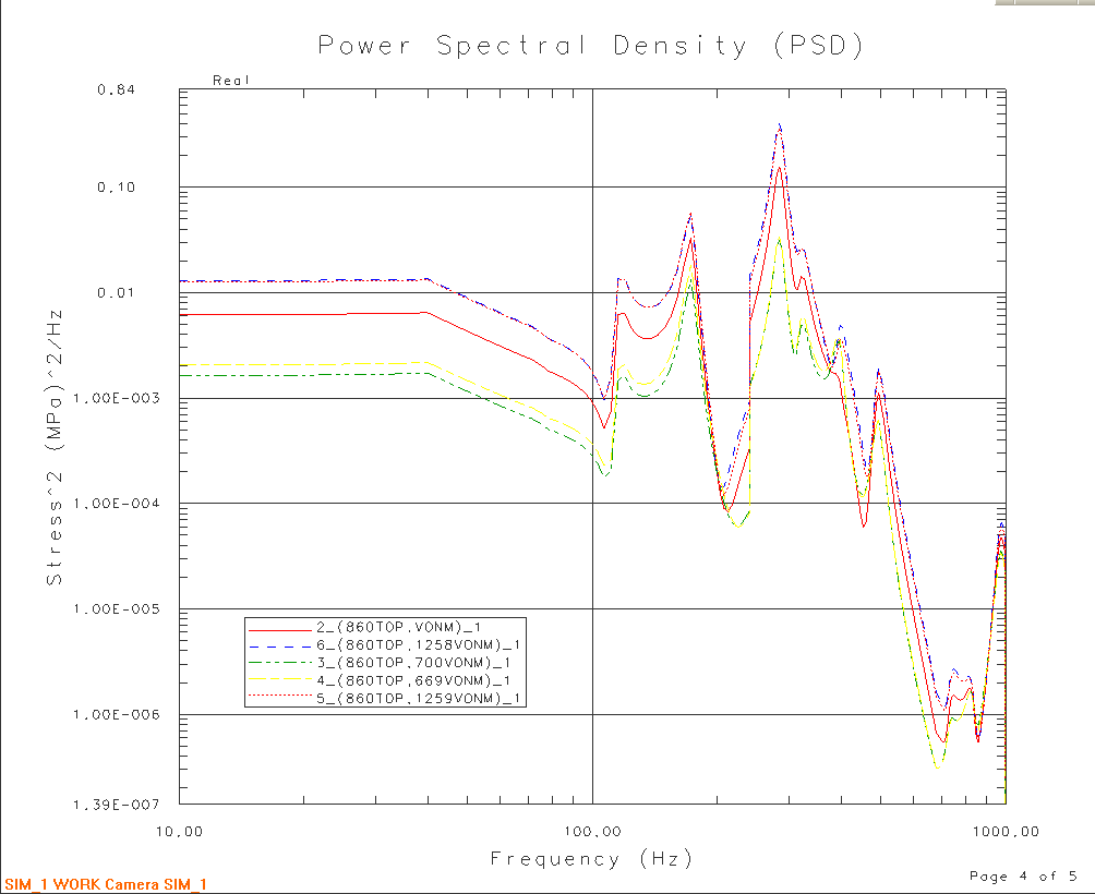
A totalof 5 functions are computed and are written to the same AFU file as the nodal result. The first is the Von Mises stress at the element centroid. Each of the other four is the Von Mises stress at one of the corner nodes of the quad element.

Compute Full Field RMS Stresses for the Random Solution

The results computed previously show the response at one location over the entire frequency range. Another way to view random results is to look at the RMS response of the full structure. This is called a full field response.

·        Select the Evaluate Contour Results icon () or right click on the event item in the Simulation Navigator and select RMS Results

·        Set the Result Type to Stress

·        Set Selection Method to ‘By Mesh’ and click on the shell mesh to select all of the shell elements.

·        Toggle on the VonMises response request

·        Select OK

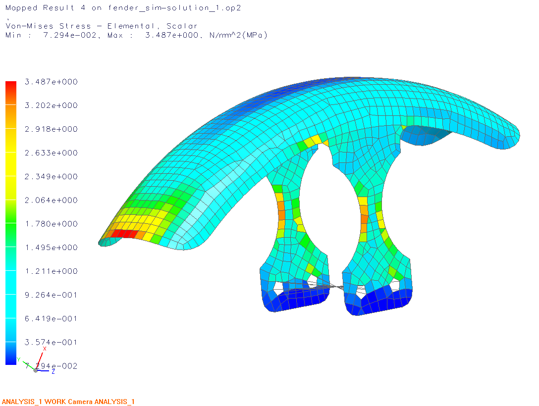
The RMS stress for all elements is computed at this time. The results listed in the Simulation Navigator under the Contour Results item and are written to an external .rs2 file. Right click on the RMS Stress item and select Post to view the result shown in the figure below.

Generate Equivalent Time Domain Solution

NX 5 includes a Java based palette of Function Tools. These tools run outside of the NX environment and can operate directly on the data in AFU files. To start the tools through NX, select Function Tools for Response Simulation () on the Response Simulation toolbar

• NOTE: If you get the following error, the UGII_JVM_LIBRARY_DIR     is not pointing to an installed Java client.

• To point to the Java client so you can start the Function     tools:

• Select File, Execute, Override Java Parameters…

• Use the Browse button to find the Java client folder on your      system

• This is typically in C:\Program       Files\Java\jre1.5.0_04\bin\client\ (the jre version may be different)

• Click ‘OK’, then select Function Tools for Response Simulation     () on the Response Simulation toolbar

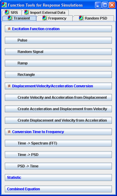
Select ‘PSD -> Time on the Transient or Random PSD tab

• Select ‘Load AFU’ and navigate to the fender_PSD.afu

• Highlight the RoadVibrationY record

• Time increment: 0.0002

• Number of Time Points: 8192(2**13)

• Interpolation Method: Log-Log

• Output Record Name: TransientRoadVibrationY

• Browse to select fender_PSD.afu as the output as well

• Click ‘OK’

The XY function Navigator in NX now shows two functions in the fender_PSD afu file

Plot the transient function

Next, check to see if the transient function adequately captures the content of the original PSD

• Select both the ‘RoadVibrationY’ and ‘TransientRoadVibrationY’     functions on the Function Navigator

• Right click and select ‘Info…’

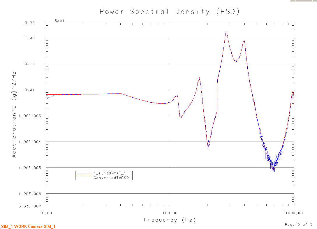
Note that the RMS values of both functions are very close. This indicates that the transient function has captured the content of the original PSD function

Evaluate Transient Response

Return to the Simulation Navigator and create a new transient event on the response simulation

• Duration: 1.6 seconds

• Note that the transient function calculated from the PSD has a      domain of 0 to 1.64 seconds

• 8192 points at 0.0002 seconds = 1.6384 seconds

• Initial Conditions: Zero

Create a new translational nodal excitation on the enforced motion grid

• Use the transient function calculated above as the excitation     in the Y direction

Evaluate the nodal acceleration response in the Y direction at the same grid as the PSD excitation was evaluated at above.

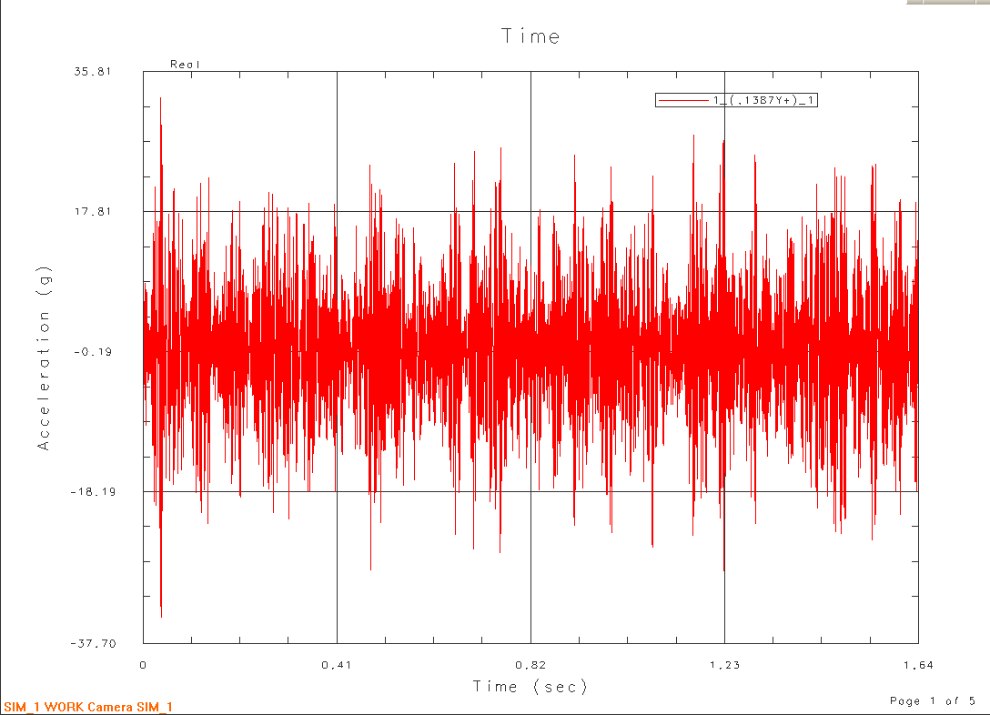
Finally, use the Function Tools to convert this transient response back to PSD and compare to the original response.

• Open the Function Tools and select ‘Time -> PSD”

• Load the AFU containing the responses for the transient event

• Select the Y acceleration record

• Enter ‘ConvertedToPSD’ as the name for the new record

• Select the transient event AFU as the destination

Select the original PSD response and the TransientToPSD record and plot them together

Adjust the X axis range to 10 to 1000 Hz.

• Toggle on the XY Plot edit mode ()

• Right click on the X axis and select ‘EditRange’

• Toggle offAutoRangeand enter     limits from 10 to 1000 Hz

Compare the RMS values of the original PSD response and the PSD response calculated from the transient response

SHAPE \* MERGEFORMAT

The calculated PSD can be “cleaned up” by using function math operations to generate a moving average

• Select Single Math () on the Function Math Operations     toolbar

• Highlight the ‘ConvertedToPSD” function in the function     navigator and select to add it to the single math selection     list

• Highlight the ConvertedToPSD function in the selection list

• Select the Moving Average operation

• Set the Moving average number to 5

• Select Append as the output

• 
  

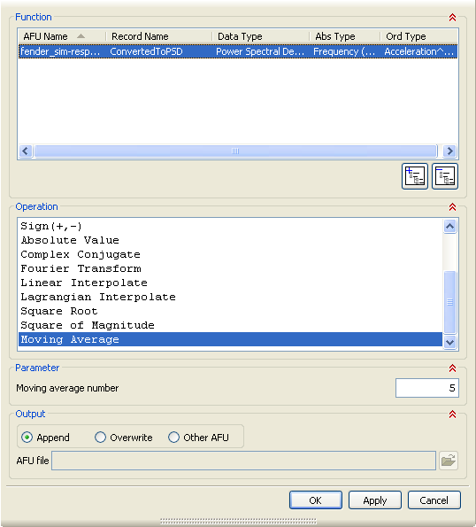
 This will create a new function (appended to the same afu file as the input) where each point is the moving average of the previous 5 points.

Plot the original PSD response and the function generated by the moving average operation

Finish

This concludes the workshop.